Maps with R (II)

Etiquetas

GeoTIFF, land cover, lattice, population, R, raster, rasterVis

In my my last post I described how to produce a multivariate choropleth map with R. Now I will show how to create a map from raster files. One of them is a factor which will group the values of the other one. Thus, once again, I will superpose several groups in the same map.

NOTE: Although the procedure described in this post is valid, there is a newer code version in one of the chapters of the book «Displaying time series, spatial and space-time data with R«

First let’s load the packages.

library(raster)
library(rasterVis)
library(colorspace)

Now, I define the geographical extent to be analyzed (approximately India and China).

ext <- extent(65, 135, 5, 55)

The first raster file is the population density in our planet, available at this NEO-NASA webpage (choose the Geo-TIFF floating option, ~25Mb). After reading the data with raster I subset the geographical extent and replace the 99999 with NA.

pop <- raster('875430rgb-167772161.0.FLOAT.TIFF')
pop <- crop(pop, ext)
pop[pop==99999] <- NA
pTotal <- levelplot(pop, zscaleLog=10, par.settings=BTCTheme)
pTotal

The second raster file is the land cover classification (available at this NEO-NASA webpage)

landClass <- raster('241243rgb-167772161.0.TIFF')
landClass <- crop(landClass, ext)

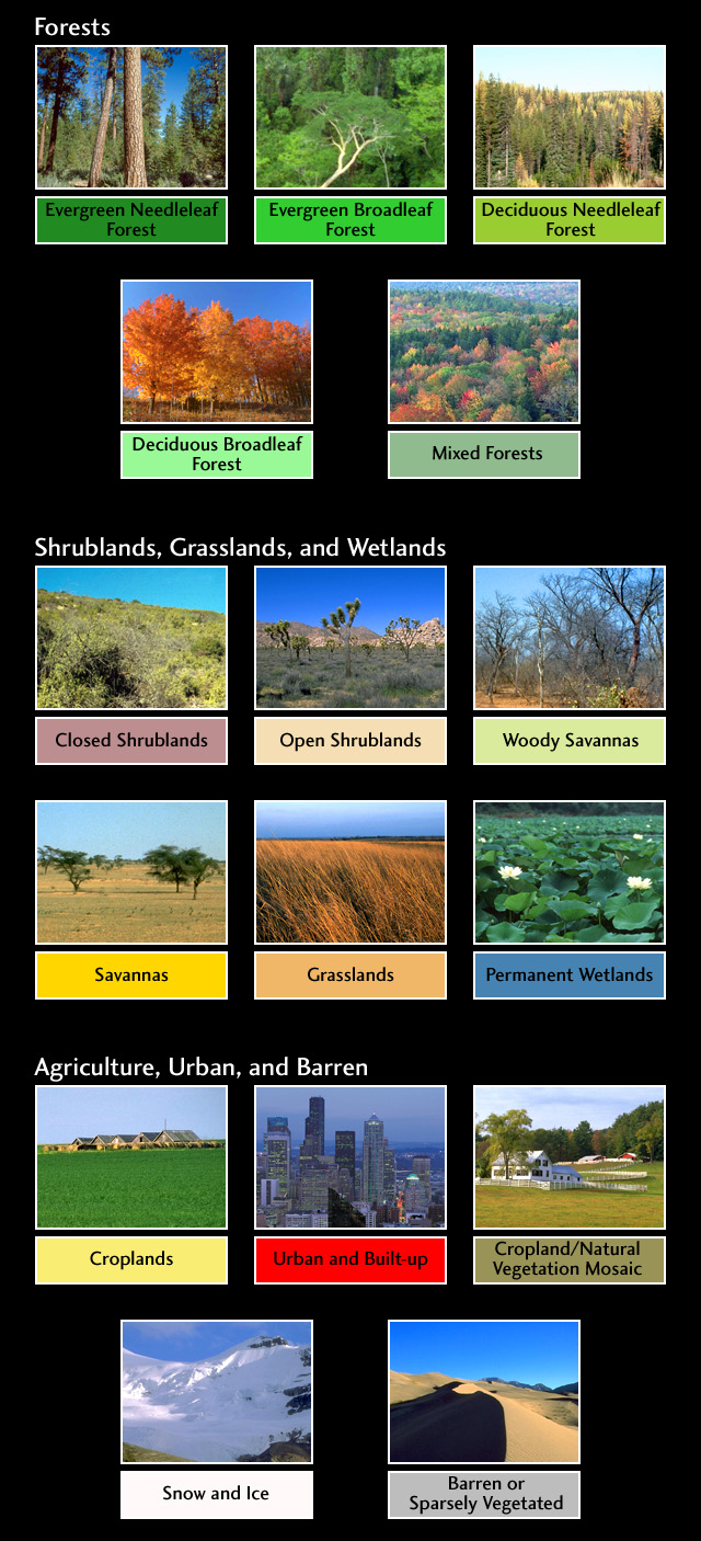
The codes of the classification are described here. In summary, the sea is labeled with 0, forests with 1 to 5, shrublands, grasslands and wetlands with 6 to 11, agriculture and urban lands with 12 to 14, and snow and barren with 15 and 16. This four groups (sea is replaced NA) will be the levels of the factor. (I am not sure if these sets of different land covers is sensible: comments from experts are welcome!)

EDIT: Following a question from a user of rasterVis I include some lines of code to display this qualitative variable in the map.
EDIT2: raster and rasterVis are able to work with categorical data using ratify.

  landClass[landClass %in% c(0, 254)] <- NA
  landClass <- cut(landClass, c(0, 5, 11, 14, 16))
  ## Add a Raster Atribute Table and define the raster as categorical data
  landClass <- ratify(landClass)
  ## Configure the RAT: first create a RAT data.frame using the
  ## levels method; second, set the values for each class (to be
  ## used by levelplot); third, assign this RAT to the raster
  ## using again levels
  rat <- levels(landClass)[[1]]
  rat$classes <- c('Forest', 'Land', 'Urban', 'Snow')
  levels(landClass) <- rat

  levelplot(landClass, col.regions=terrain_hcl(4))

This histogram shows the distribution of the population density in each land class.

s <- stack(pop, landClass)
layerNames(s) <- c('pop', 'landClass')
histogram(~log10(pop)|landClass, data=s,
            scales=list(relation='free'))

Everything is ready for the map. I will create a list of trellis objects with four elements (one for each level of the factor). Each of these objects is the representation of the population density in a particular land class. I use the same scale for all of them to allow for comparisons (the at argument of levelplot receives the correspondent at values from the global map)

at <- pTotal$legend$bottom$args$key$at

pList <- lapply(1:nClasses, function(i){
  landSub <- landClass
  landSub[!(landClass==i)] <- NA
  popSub <- mask(pop, landSub)
  step <- 360/nClasses
  pal <- rev(sequential_hcl(16, h = (30 + step*(i-1))%%360))
  pClass <- levelplot(popSub, zscaleLog=10, at=at,
                      col.regions=pal, margin=FALSE)
})

And that’s all. The rest of the code is exactly the same as in the previous post. If you execute it you will get this image (click on it for higher resolution).