More code and images from «Displaying time series, spatial and space-time data with R»

Etiquetas

github, R, spatial, spatio temporal, time series, visualization

My book continues growing. I have recently completed the first version of the Spatio-Temporal visualization chapters. Moreover, a significant part of the code of the Time Series and Spatial data chapters has been fixed and improved with new procedures and examples. The updated code is available at the github repository. Visit the webpage to explore the main images.

For example, you will find this animation:

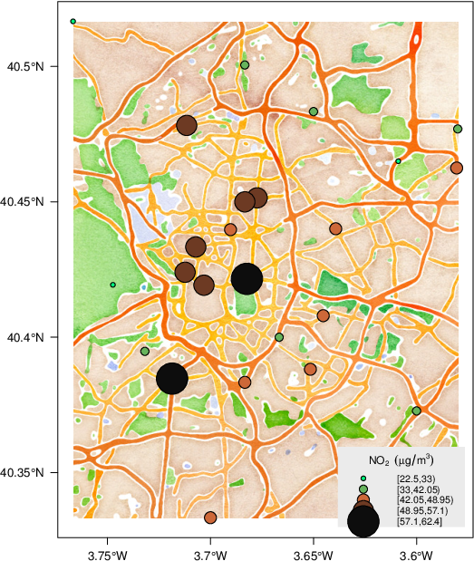
or this combination of a proportional symbol graphic with a Stamen map:

New version of solaR

Etiquetas

CRAN, photovoltaics, R, solar, solar radiation, time series

I have updated my package solaR. This package provides calculation methods of solar radiation and performance of photovoltaic systems from daily and intradaily irradiation data sources.

This last version is able to produce a synthetic daily irradiation time series from 12 monthly average values following the procedure proposed by Aguiar, Collares-Pereira and Conde, «Simple procedure for generating sequences of daily radiation values using a library of Markov transition matrices», Solar Energy, Volume 40, Issue 3, 1988.

	library(solaR)
	## Monthly averages of daily values (Wh/m2)
	G0dm <- c(2.766,3.491,4.494,5.912,6.989,7.742,7.919,7.027,5.369,3.562,2.814,2.179)*1000;
	Ta <- c(10, 14.1, 15.6, 17.2, 19.3, 21.2, 28.4, 29.9, 24.3, 18.2, 17.2, 15.2)
	g0 <- calcG0(lat=37.2, modeRad='aguiar', dataRad=G0dm)
	xyplot(g0)

view raw solaR36.R hosted with ❤ by GitHub

On the other hand, there is a new function named writeSolar to export the results of the set of functions of this package.

Happy Birthday rasterVis!

Two years ago the first version of rasterVis was submitted to R-Forge and some weeks after the first stable version was published at CRAN. My birthday gift is the version 0.21 recently available at CRAN. This new version includes several bug fixes and some code and documentation improvements:

• levelplot is able to work correctly with multivariate RATs.
• The levelplot help page has been corrected, expanded and completed with new examples.
• I have compiled a collection of questions posted to stackoverflow and R-Sig-Geo and now there is a FAQs web page.

Enjoy!

Preguntar, cooperar, investigar

Etiquetas

ciencia abierta, cooperación, docencia, EOI, investigación, procomun, software libre

Hace unos días publiqué a través de la EOI un artículo en uno de los blogs de El País. Con el título «Preguntar, cooperar, investigar» converso sobre aprender a preguntar, la investigación como proceso colectivo y la ciencia e investigación abiertas. Se puede leer aquí.

Stamen maps with spplot

Etiquetas

ggmap, ggplot2, google map, maps, openstreetmap, photovoltaics, proportional symbol, R, spplot, stamen

Several R packages provide an interface to query map services (Google Maps, Stamen Maps or OpenStreetMap) to obtain raster images from them. As far as I know, there are three packages devoted to this task: RgoogleMaps, OpenStreetMap and ggmap. The latter two are increasingly popular with a wide collection of providers.

Both of them use the background image to configure the graphical window defining functions (automap and ggmap, respectively) to display the images with ggplot2. Additional information can be layered upon this background image with ggplot2 functions. In my opinion, this approach is somewhat strange. I feel more comfortable with the approach implemented in the spplot function of the sp package, which relies on the main data to be displayed to configure the graphical window instead of using an auxiliary image as the starting point.

Although none of these two packages include functions to work with spplot, it is not difficult to build a mixed solution. The key point is that the result of their queries is mainly a raster image which can be easily displayed with the grid.raster function after some corrections.

The next code displays the location of the photovoltaic systems installed in California grouped by nominal power using data available from the OpenPV project. The procedure is:

• Download the data and define the coordinates and projection.
• Download an image from the Stamen Maps service according to the spatial extent of the data (this example uses ggmap but a similar approach can be followed with the OpenStreetMap package).
• Use grid.raster to display the image using the coordinates of its corners to define the width, height and center location.
• Display the variable with circles of different sizes and colours over the background image.

	library(sp)
	library(ggmap)
	library(RColorBrewer)
	## Get data from OpenPV. Open this URL:
	## https://openpv.nrel.gov/search?&state=CA&minsize=100&maxsize=30600&pagenum=1&nppage=25
	## and export the results as a CSV file named "californiaOpenPV.csv"
	caPV <- read.csv('californiaOpenPV.csv')
	## Longitude and Latitude are the names of columns where the spatial information is stored.
	## With the coordinates<- method caPV is now an SpatialPointsDataFrame
	coordinates(caPV) <- ~ Longitude + Latitude
	proj4string(caPV) <- CRS("+proj=longlat +datum=WGS84")
	names(caPV)[3] <- 'Pdc.kW'
	## Download stamen tiles using the bounding box of the SpatialPointsDataFrame object
	bbPoints <- bbox(caPV)
	gmap <- get_map(c(bbPoints), maptype='watercolor', source='stamen', crop=FALSE)
	## http://spatialreference.org/ref/sr-org/6864/
	## Bounding box of the map to resize and position the image with grid.raster
	bbMap <- attr(gmap, 'bb')
	latCenter <- with(bbMap, ll.lat + ur.lat)/2
	lonCenter <- with(bbMap, ll.lon + ur.lon)/2
	height <- with(bbMap, ur.lat – ll.lat)
	width <- with(bbMap, ur.lon – ll.lon)
	## Use sp.layout of spplot: a list with the name of the function
	## ('grid.raster') and its arguments
	sp.raster <- list('grid.raster', gmap,
	x=lonCenter, y=latCenter,
	width=width, height=height,
	default.units='native')
	## Define classes and sizes of the circle for each class
	breaks <- c(100, 200, 500, 1e3, 25e3)
	classes <- cut(caPV$Pdc.kW, breaks)
	meds <- tapply(caPV$Pdc.kW, classes, FUN=median)
	sizes <- (meds/max(meds))^0.57 * 1.8
	## Finally, the spplot function
	spplot(caPV["Pdc.kW"],
	cuts = breaks,
	col.regions=brewer.pal(n=5, 'Greens'),
	cex=sizes,
	edge.col='black', alpha=0.7,
	scales=list(draw=TRUE), key.space='right',
	sp.layout=sp.raster)

view raw

stamen.R

hosted with ❤ by GitHub